Molecular dynamics
This application integrates the Dynamics rust library for molecular dynamics. It's developed concurrently with this application, and the two are designed to interact. See its readme for details and assumptions. We also integrate ab-inito molecular dynamics by interfacing with Orca, if it's installed and available on the PATH. These computations are much slower, but are more accurate than Newtonian ones.
Molecular dynamics in this application is based on Amber force fields. These are Newtonian fields that are tuned for specific molecule categories (DNA, RNA, small organic molecules etc), and assume unbreakable covalent bonds. We organize these forces into the following discrete categories
Bonded:
- Bond stretching between each pair of covalently-bonded atoms.
- Angle bending, between every set of 3 linearly covalently-bonded atoms.
- Dihedral forces (AKA Torsions), between every set of 4 linearly covalently-bonded atoms.
- Improper dihedral forces between certain sets of 4 atoms in hub-and-spoke configurations.
Non-bonded:
- Lennard Jones interactions
- Short-range Coulomb interactions
- Long-range SPME Coulomb interactions
It integrates the following Amber parameter sets: - Small organic molecules, e.g. ligands: General Amber Force Fields: GAFF2 - Protein/AA: FF19SB - Nucleic acids: OL24 and RNA/OL3 libraries - Lipids: Lipid21 - Carbohydrates: GLYCAM_06j - Water: OPC
In the case of both proteins and nucleic acids, the baseline bonded and Lennard Jones parameters come from Amber's Parm19.dat, with overrides from frcmod.ff19SB and ff-nucleic-OL24.frcmod for these categories respectively.
We plan to support carbohydrates in the future.
Running MD
To run an MD computation, make sure the Dynamics toolbar is activated. Using the Sidebar, select one or more molecules to compute MD on, using the MD Button. If the molecule is selected, this button will be highlighted. If at least one protein, and at least one small organic molecule is selected, more options will display, like making only protein atoms near the small molecule dynamic. If no molecules are selected, the simulation will be of water only, with a cubical sim box with edge length twice the width of the selected solvent pad UI item. For example:
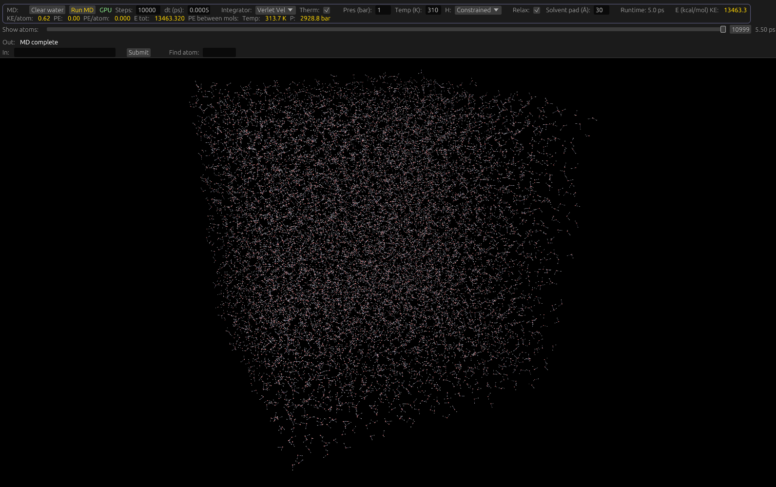
The simulation will compute in the background, but expect the GUI to be sluggish while it's running. You may abort the run at any point by clicking the Abort button which appears while a run is active. You can monitor the number of steps completed in the GUI as well.
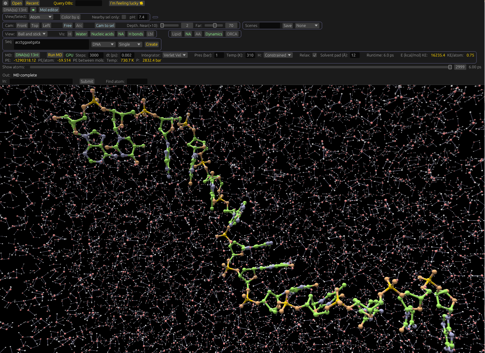
Playing back the simulation.
Once a simulation is complete, you may navigate through its snapshots by clicking, or dragging the slider which appears upon completion.
Usage details
These general parameters do not need to be loaded externally; they provide the information needed to perform dynamics with any amino acid sequence, and provide a baseline for dynamics of small organic molecules.
For small organic molecules, we may compute force field types, partial charges, and dihedral overrides. These can be provided directly from FRCMOD files, or suitably annotated Mol2 or SDF files, but are often absent. The computations we use are similar in principle to Amber's Antechamber tool, and we use parameters from it.
For details on how this parameterized approach works, see the Amber Reference Manual. Section 3 and 15 are of particular interest regarding force field parameters.
Moleucule-specific overrides to these general parameters can be loaded from .frcmod, prmptom, and .dat files. We delegate this to the bio files library, or compute them directly if not present.
We load partial charges for ligands from mol2, sdf, and pdbqt files. Protein dynamics and water can be simulated using parameters built-in to the program (The Amber one above). Simulating ligands requires the loaded file (e.g. mol2) include partial charges. We recommend including ligand-specific override files as well, e.g. to load dihedral angles from .frcmod that aren't present in Gaff2.
The algorithm
This application uses a traditional MD workflow. We use the following components:
Integrators, thermostats, barostats
We provide a Velocity-Verlet integrator. It can be used with a stochastic cell rescaling barostat (Similar to GROMACS' pcoupl = C-rescale, and either a CSVR, or Langevin Middle thermostat. Or, use the Velocity Verlet integrator without a thermostat. These continuously update atom velocities (for molecules and solvents) to match target pressure and temperatures. You can select the target temperature to the right of the integrator selector.
The Verlet Velocity integrator can be either used with CSVR thermostat, or without; this is selected using the thermostat checkbox next to the integrator selector. At this time, the thermostat temperature constant, τ, is hard-coded to be 0.9ps. Lower values correct more aggressively.
The Langevin Middle integrator is selected by default, and is always used with a thermostat. Its coefficient γ is selectable in the UI, next to the integrator selector, and is in 1/ps. Higher γ values correct to the target temperature more aggressively.
Solvation
We use an explicit water solvation model: A 4-point rigid OPC model, with a point partial charge on each Hydrogen, and a M (or EP) point offset from the Oxygen.
We use the SETTLE algorithm to maintain rigidity, while applying forces to each atom. Only the Oxygen atom carries a Lennard Jones(LJ) force. Solvation is set up by default, and requires no special adjustments. If you wish, you may change the size of the simulation box padding with its associated input on the MD toolbar.
The simulation box uses periodic boundary conditions: When a water molecule exits one side of it, it simultaneously re-appears on the opposite side. Further, our long-range SPME computations are designed to incorporate this periodic boundary position, simulating an infinitely-extending simulation box. Note that this has an unfortunate (But usually negligible) side effect of also including images of non-water molecules in computations.
Equilibration
Prior to the simulation properly starting, we perform equilibration with two techniques: Iterative energy minimization of the (non-water) molecules, and running a short simulation of only the water molecules. The minimization helps to relieve tension in the initial atom configuration. For example, if the bond length provided by the initial atom coordinates doesn't match that of the bonded length parameter.
The water pre-simulation breaks the initial crystal lattice configuration, builds hydrogen bond networks, and allows the simulation to settle at the specific temperature. We initialize water molecules with appropriate velocities, but this additional step helps. When the snapshots (aka trajectories) start building, the system will be equilibrated.
You can disable the energy minimization using the relax check box in the UI, but the water equilibration is always active. It runs in the range of a few hundred to 1,000 steps, and uses a more aggressive thermostat coefficient (τ for CSVR, and γ for Langevin) than is used during the normal simulation.
Bonded forces
We use Amber-style spring-based forces to maintain covalent bonds. We maintain the following parameters:
- Bond length between each covalently-bonded atom pair
- Angle (sometimes called valence angle) between each 3-atom line of covalently-bonded atoms. (4atoms, 2 bonds)
- Dihedral (aka torsion) angles between each 4-atom line of covalently-bonded atoms. (4 atoms, 3 bonds). These usually have rotational symmetry of 2 or 3 values which are stable.
- Improper Dihedral angles between 4-atoms in a hub-and-spoke configuration. These, for example, maintain stability
- where rings meet other parts of the molecule, or other rings.
Non-bonded forces
These are Coulomb and Lennard Jones (LJ) interactions. These make up the large majority of computational effort. Coulomb forces represent electric forces occurring from dipoles and similar effects, or ions. We use atom-centered pre-computed partial charges for these. They occur within a molecule, between molecules, and between molecules and solvents.
We use a neighbors list (Sometimes called Verlet neighbors; not directly related to the Verlet integrator) to reduce computational effort. We use the SPME Ewald approximation to reduce computation time. This algorithm is suited for periodic boundary conditions, which we use for the solvent.
We use Amber's scaling and exclusion rules: LJ and Coulomb force is reduced between atoms separated by 1 and 2 covalent bonds, and skipped between atoms separated by 3 covalent bonds.
We have two modes of handling Hydrogen in bonded forces: The same as other atoms, and rigid, with position maintained using SHAKE and RATTLE algorithms. The latter allows for stability under higher timesteps. (e.g. 2ps)
Center-of-mass drift removal
Periodically we remove any linear and angular center of mass drift, that applies to the whole system. This helps reduce extra energy in the system that may have entered from numerical precision and other error sources. We apply this to both water, and non-water molecules.
Velocity initiation and maintenance
Water molecules are initiated with velocities according to the Maxwell-Boltzmann distribution, according to the prescribed target temperature. This temperature is specified in the UI. Prior to our proper simulation start time, we briefly perform MD on water molecules only, holding the solute rigid. This allows hydrogen bond networks to form, and lets the thermostat fine-tune the velocities.
Partial Charges
For proteins, nucleic acids, and lipids, we use partial charges provided by Amber force fields (listed above) directly.
For small organic molecules, we infer AM1-BCC partial charges for each molecule when loading it. We do so using a machine learning algorithm trained on Amber's Geostd set. We use the candle library's neural nets. It's trained on this set of ~30k small organic molecules that have force field types, and partial charges assigned using AM1-BCC computations. Inference is fast, typically taking a few milliseconds.
If your small molecule already has partial charges, we use those directly instead of computing new ones. Partial charges may be provided in Mol2 files as part of their column data, or as SDF metadata. For the latter, we support both OpenFF's "atom.dprop.PartialCharge", and Pubchem's "PUBCHEM_MMFF94_PARTIAL_CHARGES" formats.
If ORCA is installed, you can use it to generate MBIS charges. This is one of the most accurate approaches, but is very slow; it may take several minutes to complete for a single small molecule. To use this, click Assign MBIS q from the ORCA UI section; it will update charges for the active molecule. You may then save this to Mol2 or SDF format if you wish. When saving to SDF, we use the Pubchem metadata format
for partial charges.
Bonded parameter overrides for small organic molecules
Small organic molecules use bonded parameters from Amber's Gaff2 set. Most molecules have dihedral parameters (proper and improper) that are not present in Gaff2. We substitute Gaff2 parameters in for these based on the closest match of their force field types to parameters present in Gaff2. We (rarely) do the same for missing bond and valence angle parameters. Alternatively, you may provide these overrides directly by opening FRDMOD or PRMPTOP files directly.
Floating point precision
This application uses mixed precision: 32-bit floating point is the default for most operations. We use 64-bit for accumulation computations (e.g. kinetic and potential energy), and in thermostat and barostat computations. The use of 32-bit floating point introduces more precision errors than 64-bit, but reduces memory and bandwidth cost. This is especially relevant for parallel computations: The CPU can perform twice as many 32-bit SIMD operations are 64-bit, and bandwidth to and from the GPU on the PCIe bus is halved. Perhaps more importantly, consumer GPUs have poor f64 performance, so using 32-bit values significantly improves speed on these devices.
How pH adjustment works
pH in proteins is represented by the protenation state of certain amino acids. In particular, His, Asp, Cys, Glu, and Lys are affected. These changes are affected in utility functions we provide that add Hydrogen atoms.
Saving results (trajectories))
Snapshots of results can be returned in memory, or saved to disk in DCD, TRR, and XTC, or TRR formats.
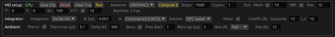
Formats are selected prior to an MD run, in the MD setup parameters. You can select which formats to enable with checkboxes in the UI. Once selected, you can set the ratio at which snapshots will save in that format. You can then select the ratio used by each format. I.e., save snapshots that often for each format. For TRR, you can specify ratios for coordinates, velocities, and forces separately. By default, this files will save in the Molchanica working directory, in the md_out subfolder. A new file will be created for each MD run, and for each trajectory format. It will be periodically written as the simulation runs.
Both the Dynamics and GROMACS backends support these settings.
Here's a summary of the formats, which may help you select which to use:
- TRR: A digital format which contains full-precision data as combinations of coordinates, velocities, and forces. Used by GROMACS.
- XTC: A digital format which contains compressed coordinates. Used by GROMACS.
- DCD: A digital format which contains full-quality coordinates. Used by CHARMM, NAMD, and OpenMM.
To save and load in XTC format when using the dynamics backend, you must have the MDTraj program installed and available on the system PATH. This can be installed with pip install mdtraj or using conda. The DCD and MDT (native) formats do not have this requirement.
GROMACS dos not support the DCD format.
We store energy in a separate format: GROMACS' EDR.
More information
We plan to support carbohydrates and lipids later. If you're interested in these, please add a Github Issue.
These general parameters do not need to be loaded externally; they provide the information needed to perform MD with any amino acid sequence, and provide a baseline for dynamics of small organic molecules.
This program can automatically load ligands with Amber parameters, for the Amber Geostd set. This includes many common small organic molecules with force field parameters, and partial charges included. It can infer these from the protein loaded, or be queried by identifier.
You can load these molecules with parameters directly from the GUI by typing the identifier. If you load an SDF molecule, the program may be able to automatically update it using Amber parameters and partial charges.
For details on how dynamics using this parameterized approach works, see the Amber Reference Manual. Section 3 and 15 are of particular interest, regarding force field parameters.
We load partial charges for ligands from mol2, PDBQT etc files. Protein dynamics and water can be simulated using parameters built-in to the program (The Amber one above). For small organic molecules, we infer force field params, and partial charges for each atom, as well as molecule-specific frcmod overrides from GAFF2: Generally, this is proper and improper dihedral angles. It is, occasionally, bond and angle parameters.
You can load (and save) combined atom and forcefield data from Amber PRMTOP files; these combine these two data types into one file.
Use the code below, the Examples folder on Github, and the API documentation to learn how to use it. General workflow:
-Create a MdState struct with MdState::new().
This accepts a configuration, the molecules to simulate,
and force field parameters.
Run a simulation step by calling MdState::step(). This accepts an enum which defines the computation devices
(CPU/GPU), and the time step in picoseconds. This step can be called as required for your application. For example
you can call it repeatedly in a loop, or as required, e.g. to not block a GUI, or for interactive MD.
Energy, temperature, and pressure measurements
With a given snapshot selected, the MD toolbar displays instantaneous measurements of energy, temperature, and pressure at that snapshot. Potential energy is broken down into two components: That from covalent bonds (Bonded), and that from Coulomb, Lennard Jones, and SPME forces. (Non-bonded) These values all take into account both the molecules loaded, and the explicit water solvent molecules. Water molecules are treated as any other, with some exceptions due to their rigidly-defined geometry.
Kinetic energy is computed using the standard manner: By computing the mass of each atom multiplied by the magnitude squared of its velocity, summed over every atom. Temperature, displayed in Kelvin, is computed as follows: $2 KE / (DOF × R) $ , where R is the Boltzmann gas constant, defined as 1.987 × 10³ kcal mol⁻¹ K⁻¹. (These are the simulation's native units).
DOF is the number of degrees-of-freedom of the system. We compute this as 3 × the number of non-static atoms in the system excluding water, for the 3 orthogonal directions an atom can move. We add 6 × the number of water molecules in the system; this takes into account its rigid character, with each water molecule having 3 positional degrees of freedom, and 3 rotational ones. We subtract one degree of freedom for each non-water hydrogen atom, if hydrogens are set as constrained. We also subtract 3 DOF for the center-of-motion drift removal, and 3 for its angular motion removal.
Saving and loading MD configuration
You can save and load MD configuration in GROMACS format. To save, click the Save MD button in the MD toolbar. This will save 3 files to the folder you select:
.mdpConfiguration data. The integrator, constraints, time step, sim box, and many more items..gro: Positions, force field names, and other information for each atom in the simulation..top: Force field parameters for each atom, bond, and set of 3 and 4 adjacent bonds. This includes both bonded and non-bonded forces, as well as rigid constraints, for example on molecules. Also includes SETTLE constraints for solvents, and anything else which defines force fields.
To load these, use the standard file opening functionality you use for molecules. E.g. use the open button, or drag the file into the window. These will, like other file types show up in the open history.
Selecting a backend
If GROMACS or ORCA are available on the system, you a Backend dropdown will appear. You can use this to change the MD engine in use. This operation is intended to be transparent between Dynamics (Our own engine), and GROMACS, although ORCA's MD capabilities and configuration are very different from these, and are only suitable for small systems.
ORCA
If Orca is installed and available on your system's PATH environment variable, we can perform Ab initio molecular dynamics using it. The computations are run entirely from Orca, with Molchanica providing its input from GUI interactions, and collect and display its output.
See This ORCA documentation page for details on these computations.
To use this functionality, enable the ORCA toolkit by clicking its button in the UI. This will open a set of commands for applying MD on the active molecule. From here you can select the computation method/functional, basis set, and other options. Click Run Ab-initio MD to run. Note that this takes much longer to run than our native MD computations, but is more accurate.